The Shadow Public is a video installation exploring the concept of “the public” in visual culture.
Digitized American movies from the 1950s and 1960s are selected from the Internet Archive. A moving-image collage is then produced algorithmically, using a technique based on the Gram-Schmidt procedure. The result is a collective portrayal of the construction of the category of the public in American culture during those years. In particular, the aim is to explore the relationship between two core themes “history from above” and “history from below”.
CONCEPT
The Internet Archive (IA) is a digital library that contains several public domain collections of American digitized videos, text documents, and other materials.
For this project, we have selected video material based on two sets of topics.
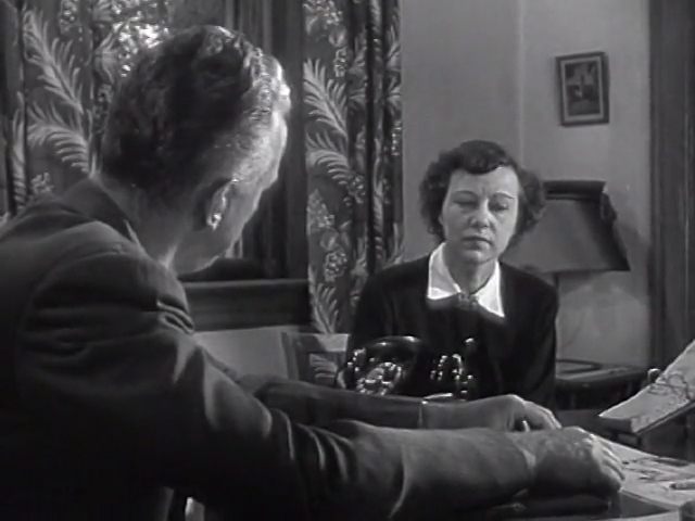
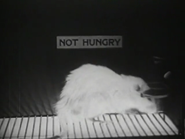
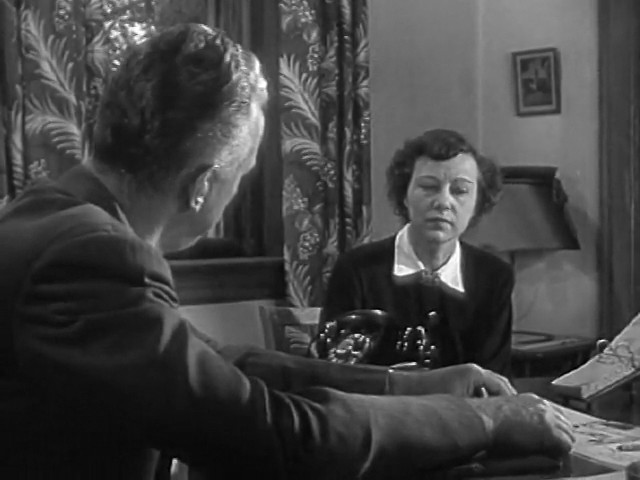
The first set includes primarily videos associated with the topics of “social guidance”, “education” and “psychology”. Many of these videos include public education films, often produced by the government or by large corporations. They express attempts by authorities to construct a concept of the public and the subject’s role within it. They were made to construct docile, obedient citizens. (1) Some of these videos aim to identify social problems, for instance anger, depression, etc. Others explain dominant theories of human and animal psychology. We can think of these videos as a history from above, one that express hegemonic ideas. We also included educational films about animals and about science, since the image of the public constructed from above is often justified by appeals to science (for instance cybernetics).
The second set consists of IA videos associated with the “home movies” topic. We can think of these videos as a history from below, one that is produced by the people. These home movies capture many aspects of the texture of everyday life. Home movies express a conception of the public that is not bound by dominant social categories, a vision of shadow publics beyond official history. They perform a “redemption” of the texture of daily reality. (2)
Selected videos are then collaged using a specially-designed algorithm.
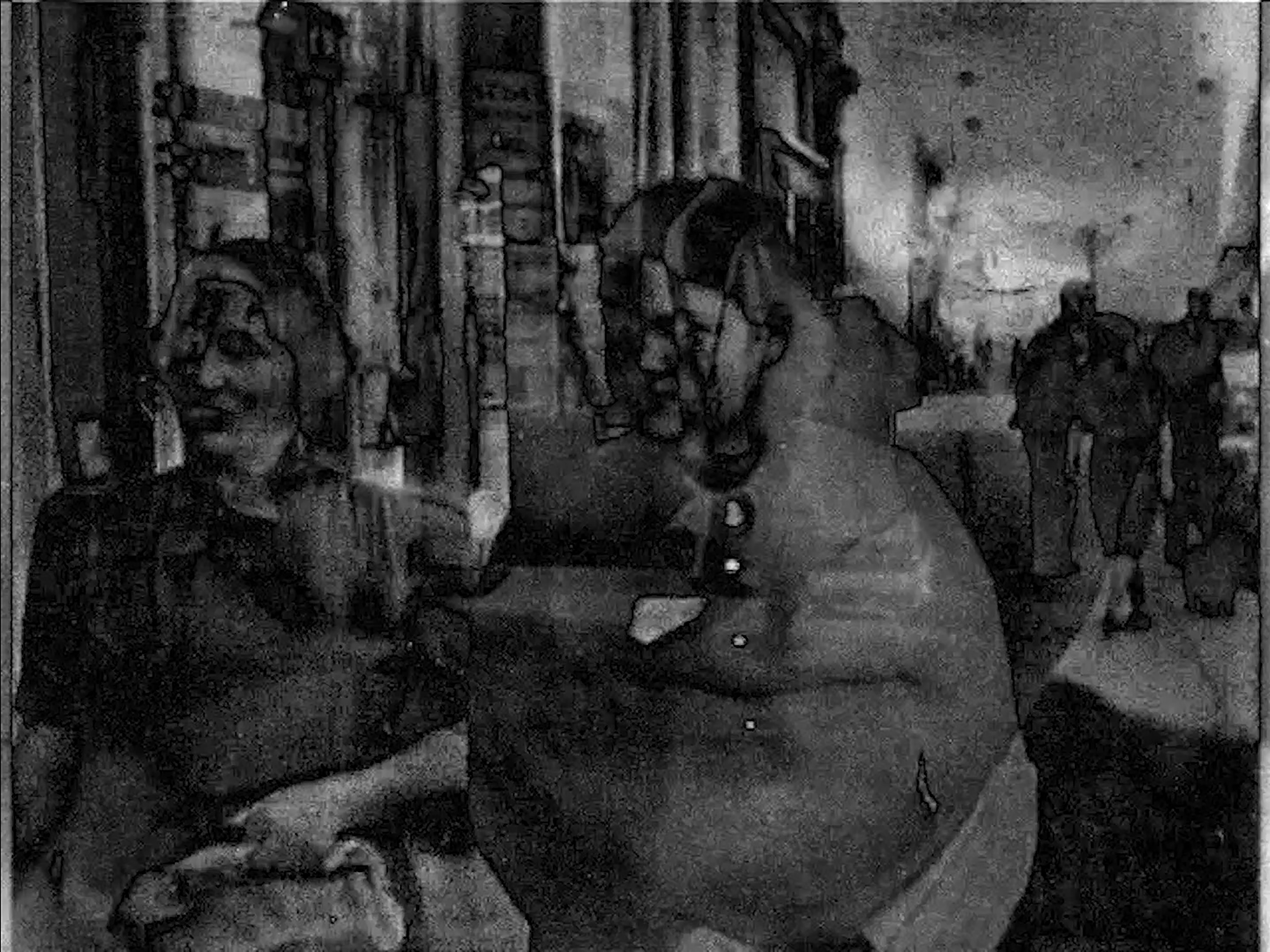
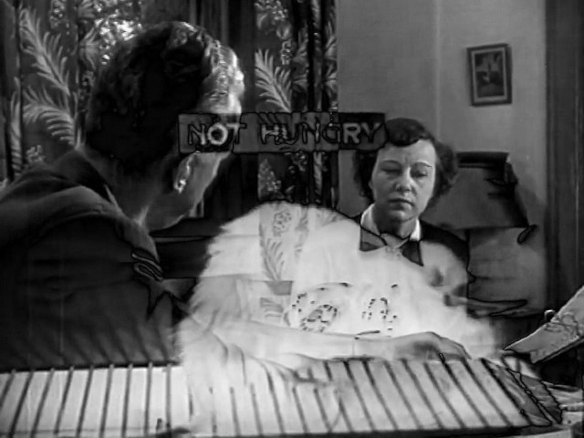
The procedure processes and recombines video images based on the brightness of their pixels rather than any thematic contents. It can establish fresh, unpredictable thematic connections among different videos, freed from any prior messages or ideas. For instance, the procedure juxtaposes images of children in home movies with images from scientific experiments involving animals. We can think of this collage technique as the automatic construction of visual figures (visual analogies, metaphors, and connections), which were not planned by the artist. It thus generates potentially novels points of view on the video data.
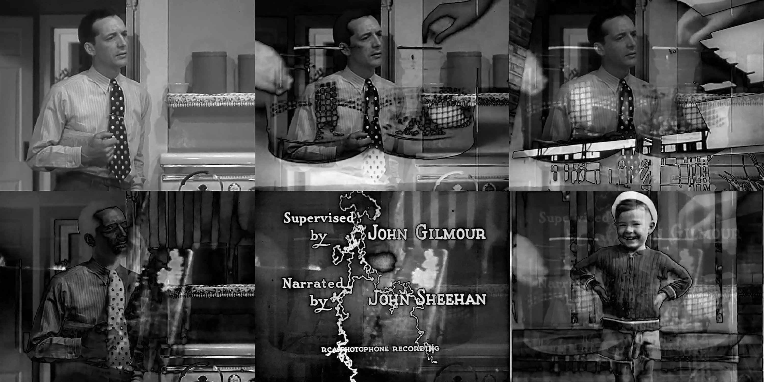
The work can be shown as a single image (see the video on top of this page) or as a grid:
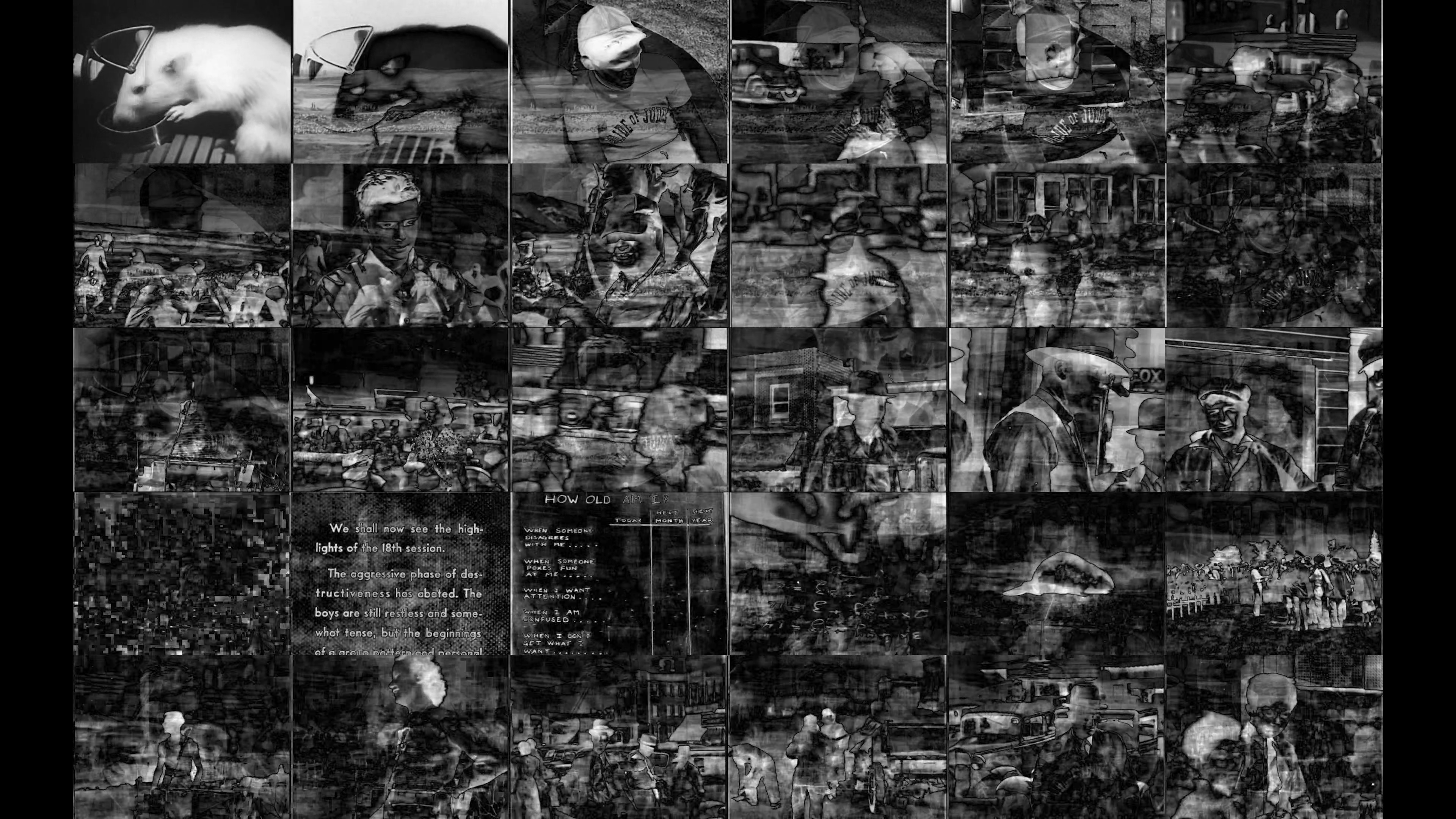
This grid is generated by an algorithm that starts from a single base image and then continues producing visual collages by introducing various new images from the available collection. The grid shows, from left to right and top to bottom, several iterations. The advantage of the grid method is that the generative method is, if not entirely transparent, at least referenced obliquely by the multi-screen presentation. The visual grid highlights that every image in the culture is understood in relation to other images.
The grid presentation can be extended, if there is a large screen available, since the visual collage technique developed here imposes no limitations on the size of the visual matrix.
The choice of home movies from the 50s and 60s precedes the development of social video sharing platforms, where success is often measured in terms of the quantity of views and audience experience is mediated by advertisements. Older home movies were not produced for potential mass consumption and so remained relatively marginal within the hegemonic structure of production and distribution.
_____________
(1) The theme of the construction of obedient citizens has been explored in: Toby Miller, The Well-Tempered Self: Citizenship, Culture, and the Postmodern Subject, Baltimore: John Hopkins University Press, 1993.
(2) The concept of redemption has sometimes been associated with the medium of cinema itself. One author claims that cinematic images redeem everyday reality. See: Sigfried Kracauer, Theory of Film: The redemption of Physical Reality, Princeton, 1998.
Setup
The presentation format can be adapted to the available resources. If only a monitor is available, the work can be shown as a single movie.
If a video projection can be arranged on a large screen, it would be better to show a grid containing multiple collages in a single channel. The grid can be projected as a single-channel video, but needs a large screen so that details can be appreciated. (See the technical description session for a description of the method that produces multiple collages.)
If there is a large projection surface available, the larger grid version can be shown.
All formats involve pre-rendered videos, which can be played with a computer, so it is very simple to set up this work.
FORMAT
Resolution: Full HD (1920x1080) for grid version or 480p (640x480) for single version
Video format: MPEG4
Codex: H.264
Color: black an white
Sound: Silent
The grid version of the work requires one ceiling-mounted projector
(Full HD resoultion and minimum 3000 ANSI Lumens)
BACKGROUND
Several tasks in image processing and analysis, such as for instance segmentation, classification, or edge detection, can be tackled by applying various filers to the image under consideration. The filters are designed to respond to the presence of the features of interest (e.g. edges or corners) in the image.
Just as an audio waveform can be decomposed into elementary sinusoids (simple sine and cosine waves) of specific frequencies, an image can be decomposed into elementary patterns of bands (2D sinusoids). The weights of these different frequency components in any given image account for many visual properties of the image. Edge detection filters can be designed to respond to oriented elements (e.g., horizontal, diagonal, or vertical boundaries) and so can be used to analyze the visual structure of the image.
The following filter, for example, detects vertical edges.
A question that arises in this context is the identification of the best filters for one or more given tasks. A widely used criterion for a good filter is that it should minimize the uncertainty of the description that results from applying it to any given image.
What does uncertainty mean here? In everyday life, we might say things like “Pedro arrived at 6 O’clock, give or take ten minutes”. The expression “give or take” indicates the uncertainty of our knowledge. We do not give a specific time but rather a range or interval. We can think of the word “uncertainty” as an expression of this “give or take” property that pervades our knowledge of the physical world. To speak of uncertainty is to speak of limits to the achievable resolution in our information about a specific kind of signal.
In the case of images, we are interested in identifying edges and their orientations. This aim is accomplished by describing the visual frequencies detectable in specific locations in the image. To tackle this problem is to think of an image from two different viewpoints. First of all, the image is viewed as a set of discrete positions (pixels), each with a certain brightness. Secondly, the image is also viewed as a combination of sinusoidal plane waves. We want to represent the image in both the space domain and the frequency domain, and so to adopt both viewpoints at once. Thus we wish to obtain information with the least possible uncertainty concerning frequency and position.
Frequency uncertainty occurs when instead of detecting the intended frequency we detect a range of frequencies. Position uncertainty occurs, for instance, when an image is blurred, and so the brightness of a given pixel p is replaced with a weighted average of the brightnesses of pixels in a region centered on p.
In general, an uncertainty principle asserts the existence of limits to the precision that can be attained in our knowledge of a complementary pair of physical properties, such as the momentum and position of a particle. The uncertainty principle for still images asserts the existence of a lower bound to the joint position-frequency uncertainty in the representation of an image. Once the theoretical lower bound is attained, any further improvements in one domain (frequency or position) must be paid for with a loss of resolution in the other domain.
The so-called Gabor image filters are designed to minimize the joint position-frequency uncertainty. Different filters attain a better position resolution by sacrificing frequency resolution, or vice versa.
Every Gabor image filter has two components. The first is a blurring filter consisting of a discrete kernel that approximates a continuous Gaussian function. Its uncertainty is determined by the standard deviation of the Gaussian function (and so, by the radius of the corresponding filter). The second filter is a quadrature pair of oriented two-dimensional sinusoids that respond to certain orientations (horizontal, vertical, diagonal) and wavelengths within the image. Its uncertainty depends on the effective bandwidth of the filter. The combined uncertainty is the product of the uncertainties in the two domains. We wish to minimize this combined uncertainty.
The Gaussian components of the following horizontal filters have (from right to left) standard deviation 22.4, 11.2, 5.6, 2.8 and their respective effective bandwidths are 0.02, 0.04, 0.07, 0.14 Hz (cycles per pixel). The lower bandwidths require a higher standard deviation, and vice versa.
If we wish to identify precisely certain frequency-domain properties in an image, we need to sacrifice resolution in the position-domain, i.e., blur the image. We might then know more precisely which frequencies make a strong contribution globally to the image, but we lose precision in our knowledge of the areas of the image wherein those frequencies are active. If we wish to gain more precise location information, we need to sacrifice frequency resolution, i.e, use a filter that responds to a wider range of frequencies.
The following image shows the position-frequency trade-off. The source image is a Siemens Star, often used in video adjustment charts. As the spatial resolution of the image is decreased (as we blur the image), its Fourier representation becomes better localized in frequency.
The top row of this diagram shows the result of applying different Gaussian filters to the image.
Each column shows the application of complete Gabor filters with the same standard deviation, but with different orientations.
The second (fourth, fifth) row then visualizes the Fourier domain decomposition of the result of applying the filter to the Siemens Star picture. In general, the Fourier decomposition is more concentrated as the standard deviation of the Gaussian increases (i.e., the resolution of the decomposition improves as we move towards the right, i.e., as the resolution of the spatial information, the sharpness of the image, decreases).
The third (fifth, seventh) row is the activation pattern that results from applying a filter with a specific orientation to the source image. We can think of this as the result of the analysis.
A note on visualization. The Gabor filters are complex filters. In displaying the results, we show the amplitude spectrum, i.e., the square root of the sum of the real parts squared.
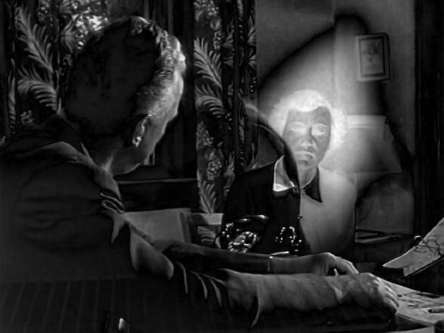
The following diagram shows several frames from Ingmar Bergman’s film Persona and the amplitude spectrum of the result of applying various Gabor filters (with different orientations and bandwidths) to those frames.
_____________
REFERENCE
John G. Daugman, "Uncertainty relation for resolution in space, spatial frequency, and orientation optimized by two-dimensional visual cortical filters", Journal of the Optical Society of. America A, 2, 1160-1169 (1985).
ALGORITHIM
This section explains the technical procedure. It is not necessary to understand this procedure in order to appreciate and evaluate this work, so this section, which assumes some basic knowledge of linear algebra, is optional.
ORTHOGONALIZATION
The core technical innovation in this project involves the repurposing of an orthogonalization procedure as a tool for video collaging. This section explains the procedure in question.
Given a set of linearly independent vectors in an inner product space V, an orthogonalization procedure outputs a new set of orthogonal vectors that span the same subspace in V. (1)
Perhaps the best-known orthogonalization procedure is the Gram-Schmidt technique. To understand this method, we need to introduce the notion of orthogonal projection.
A frame is a set of n x m pixels, where n and m are the width and height of the image. A movie is a sequence of frames.
Associated with every frame f in movie M is a function Bf (x,y) whose inputs are the screen coordinates of a specific pixel and whose output is a floating point number in the range (0, 1), the “brightness” or “value” of that pixel.
A frame f can also be described as a vector in ℝn x m whose (y * m + x)th component is given by Bf(x,y). In other words,
the vector is an array containing the values of every pixel in f. They are sequentially ordered,
so that the values of the pixels in the first row are followed by those of the pixels in the second row, and so on.
We take the set F of all frames of n x m pixels as a vector space, equipped with the two basic operations of vector addition and scalar multiplication.
We endow F with a dot product, an operation whose inputs are two vectors and whose output is a single number. The dot product of two vectors is obtained by multiplying every pair of corresponding entries and adding the results.
The expression <u1, u2> denotes the dot product of vectors u1 and u2.
Two vectors u1 and u2 in some vector space V are orthogonal (or perpendicular) if and
only if <u1, u2> = 0. The “size” or “length” of a vector u, written ‖u‖, is given by
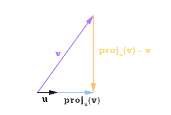
Given a vector u in F, the orthogonal projection of vector v in F onto u is defined as
We will also say that Pu (v) is the shadow cast by v on u, or the component of v in the direction of u.
The actual Gram-Schmidt procedure is simple. Given a set of linearly independent vectors v1 , v2 , v3 , ... vk in ℝn, the Gram Schmidt procedure constructs the output vectors u1 , u2 , u3 , ... uk as follows: .
u1 = v1u2 = v2 - Pu1 (v2)
u3 = v3 - Pu1 (v3) - Pu2 (v3)
u4 = v4 - Pu1 (v4) - Pu2 (v4) - Pu3 (v4)
⁝
uk = vk - Pu1 (vk) - Pu2 (vk) - ...... - Puk-1 (vk)
The Gram-Schmidt method returns the normalized vectors uk. This normalization is accomplished by dividing every uk by its vector norm.
The normalized vectors are not images. In particular, they contain negative values. To produce visible images, we first compute the maximum and minimum values for each normalized vector that results from the Gram-Schmidt procedure. We then define an operation on the nth component of the kth vector:
F(uk , n) = map( ukn , 0, max, 0, 255), if uk ≥ 0
F(uk , n) = map( ukn , min, 0, 0, 255), otherwise.
where ukn is the value of the
nth element of the kth vector produced by the
Gram-Schmidt procedure and map() is a linear mapping
function.
For instance, suppose the algorithm receives the following three images.
We would output the following three images. Note that the first output vector is always identical to the first input image.