TECHNICAL PROCEDURE

 

The basic idea of Gestus involves identifying sequences within the source film that manifest similar motions. The similarity is to be assessed not in terms of the object that moves but in terms of the speed and direction of movement. How is this to be done?

It is important to observe at this point that this problem is only vaguely defined. Experimental artists often face problems of this nature. The problem itself is not understood until its solution has been found. One cannot know in advance what counts as an appropriate solution. To find a solution is to define the very terms of the problem. The artist identifies the solution and the problem at the same time. The production of the work is not just about making a selection out of a set of possible answers, but also about coming to see or understand the problem and its possible answers differently. In social theory, this type of problem is known as a “wicked problem”. ⁽¹⁾ In a wicked problem, every attempt to identify a possible solution modifies the very understanding of the problem. Thus the definition of the problem is not predefined once and for all. Rather, its definition evolves in the course of attempting to solve it. According to this model, the artist does not know quite what is required, and so does not understand what it means to “get it right”. There is no determinate “stopping rule” that identifies the presence of a solution. The situation is essentially indeterminate. An important background to this idea is the view that persons do not typically have stable understandings of any given situation. ⁽²⁾ The artist’s achievement is to be judged not so much in virtue of their efficacy as in virtue of their proposing a new perspective that reconceptualizes the situation at hand and disclosed a new set of possibilities.

The creative process that led to the production of Gestus was mainly directed towards trying to understand, by a process of technical experimentation, the nature of the problem: what does it mean, to identify similar or “matching” movements in films? We knew that this would somehow involve the computation of optical flow, but other details were not clearly specified at the outset. The rest of this section outlines the results that have been achieved. These results take the form of an algorithm, which we now describe.

The core contributions are described in sections 2, 3, and to a lesser extent section 6.

 

1. OPTICAL FLOW

The input to the algorithm is a movie, i.e., a sequence of images or “frames” originally shot on celluloid but available in digital form. The original film was made without synchronized sound, and it contained intertitles. All intertitles have been removed manually.

Every frame consists of a two-dimensional array of grayscale pixels. Every pixel is represented by a real number, the brightness or intensity of that pixel. This paper uses the expression B(x, y, t) to denote the intensity or brightness of the pixel at location (x, y) in frame t of the movie.

As a pre-processing step, the brightness of the pixels in every frame is standardized to zero average and unit standard deviation in order to compensate for variations in illumination.

The video source also suffers from various defects due to its age. Some images are unstable, and many scratches, dust marks, and other symptoms of physical damage are visible on the image. These defects tend to produce inaccurate optical flow estimations and so need to be corrected.

To stabilize images, we perform a phase correlation on each pair of subsequent images to obtain an estimate the relative translation from one image to the other, and then use the translation vector to warp the second image in the direction of the first.

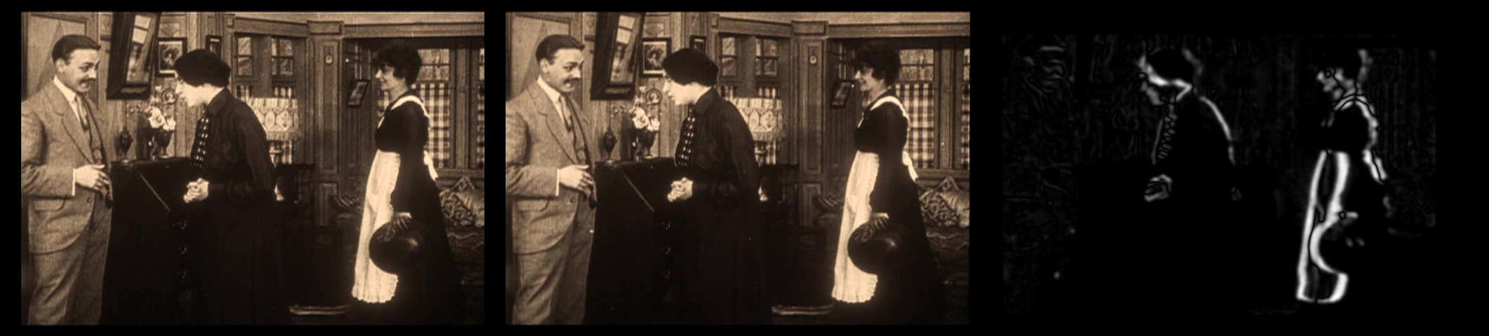
The next step involves using a threshold on the temporal gradients to further eliminate the effects of noise on the optical flow estimation. This involves computing the brightness difference between every pair of successive frames. If |B(x, y, t) – B(x, y, t+1)| < threshold, we label the pixel B(x,y,t) as static and do not track it across frames. Those pixels with a difference equal to or higher than the threshold are marked as active pixels.

This figure shows two frames and the gradient image. Points below threshold have been set to black.

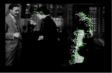
We then use a Harris corner detector to find key points among the active pixels in each frame. ⁽³⁾ The purpose of this detector is to find pixels in the image with reasonably high gradients along both spatial directions. These points are often considered particularly good to track.

Once good points have been selected, the next step is the application of an image registration algorithm to extract the optical flow for each frame. Optical flow consists of patterns of apparent motion across two images. This work uses the classical technique proposed by Lucas and Kanade. ⁽⁴⁾ The output of the algorithm associates every trackable point with a translation vector that represents its motion along the x and y directions. Note that when we speak of the optical flow of a frame, we always mean the optical flow computed between that frame and the immediately succeeding frame in the source video.

 

2. DECOMPOSITION INTO CONNECTED REGIONS

In the original version of Gestsus, the optical flow data for each frame was quantized into a matrix whose (i,j)th entry represents the number of vectors with magnitude i and direction j. This two-dimensional Flow Histogram (FH) approach worked reasonably well as a statistical representation of the optical flow in the whole image, but all information about movement in different regions of the frame was lost. The organization of movement within the frame is not well-captured. This problem manifested itself in some visually unconvincing matching results.

The new version of this project does not construct any FH. Instead, the procedure quantizes the flow vectors by imposing an N x M grid on the image and assigning to every cell in the grid the component-wise average of all flow vectors within the cell. If there are no active pixels within a cell, we assign to that cell the zero vector.

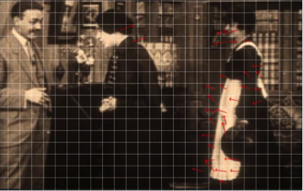
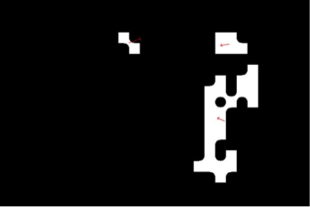
We use this grid to produce an N x M binary image where every pixel is set to zero if the grid cell contains no motion (i.e., its flow vector magnitude is zero). Otherwise, the pixel is set to 1. We treat all zero pixels as background and all others as foreground.

We then apply a morphological closing operator to the binary image, to remove small holes within the foreground and background regions. This closed binary image then becomes the input to a connected-component labeling algorithm that identifies connected foreground regions. ⁽⁵⁾

Each connected region is then associated with a representative vector, computed as the component-wise average of all flow vectors in the region.

By identifying regions within an image, we retain some information about the visual organization of movement within each frame. This point is important for aesthetic reasons. Judex, the source video, exemplifies a tradition of ‘tableau cinema’, characteristic of early silent films. This kind of cinema relied on deep space staging rather than camera movement or analytical editing. Film theorist and historian David Bordwell stresses director Louis Feuillade’s skill at forming dynamically changing geometric arrangements of bodies in space, carefully directing the viewer’s gaze to salient features of a scene on a moment-to-moment basis. “Such gentle geometries of movement hard to find in today’s cinema, and observing them in Feuillade reminds us that long ago some directors crafted their images as two-dimensional patterns of bodies in space.” ⁽⁶⁾ Bordwell has noted the rhythmic quality of cinematic motion in Feuillade’s work: “Shots are subtly balanced, then unbalanced, then rebalanced...” ⁽⁷⁾

The algorithm for this new version of Gestus has been designed to capture certain aspects of the internal organization of movement within each image. It is for this purpose that the image was broken down into regions, and each region was assigned motion vector.

 

3. COMPARING FLOW VECTORS AND IMAGES

A procedure is needed to compare optical flow vectors in order to find matching images. We assign 12 possible directions and 4 possible magnitudes for a total of 48 possible vectors. We then represent every region’s flow vector as one of those 48 vectors.

The rationale for this representation has to do with the ultimate aim of the project, which is to compare optical flow vectors in order to identify similar movements in the source movie. The representation used here gives us a natural way to define a distance between vectors.

The distance between two vectors is the minimal number of quantized steps connecting them. For instance, the two vectors highlighted below are connected by 3 steps.

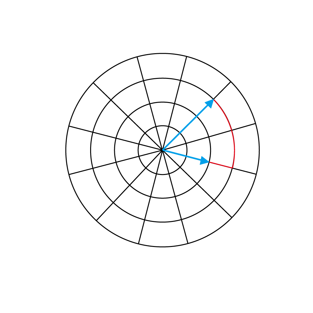
We will use the notation d(u, v) to denote the distance between two vectors. We will sometimes use the same notation to denote the distance between two image regions, computed as the distance between the two flow vectors associated with each of the two regions.

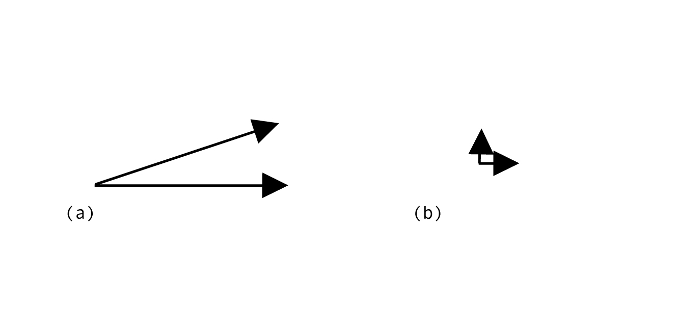
Why do we employ this measure to compare vectors? While it is common to use the Euclidean distance to compare optical flow vectors, we have avoided this choice. Authors have often remarked that the Euclidean distance does not correspond to our perceptual experience of optical flow. ⁽⁸⁾ For instance, we experience vectors (a) as more similar to one another than those in (b), but the Euclidean computation produces the opposite result. ⁽⁹⁾

Authors have proposed several alternative measures that better capture our immediate judgments of perceptual similarity among vectors. The measure we use, as described above, is based on from the Motion Retrieval Code approach proposed by Jeong and Moon. ⁽¹⁰⁾

If we wish to compare the optical flow in two distinct frames, we proceed by comparing the vectors in the regions of those frames using an adaptation of the Hausdorff distance. This measure has often been applied to pixel brightness data in image comparison and matching tasks. ⁽¹¹⁾ We extend this measure to the comparison of optical flow vectors associated with image regions.

The Hausdorff distance between any pair of frames X and Y is defined as:

where x and y vary over the regions in X and Y respectively, and d(x, y) is the distance between optical flow vectors associated with regions x and y.

 

4. SEGMENTATION

An important difference between this version of Gestus and the original version involves the segmentation of the input video. In the original version, the input video was divided into segments of uniform length. In this version, the segmentation procedure produces segments of variable length. We find it very important to divide the movie into segments according to natural change points.

Variable-length segmentation tends to produce more perceptually compelling matches than fixed-length segmentation, which often produces arbitrary change points.

Given the input video, we first make a very rough segmentation into clips by detecting larger than threshold changes in the average brightness across two frames. Each clip is then segmented more finely using a simple sliding window technique to detect change points. The technique has two parameters, the minimum segment size m and the maximum segment size n. We begin processing the first frame of the video by selecting m consecutive frames as our initial segment. We then compute the Hausdorff distance (section 3) of the last frame in the segment to the next frame in the video. We repeat the procedure, growing the segment by one frame until we have reached a segment with n frames. We then select the frame with the smallest distance as the breakpoint. We then repeat the procedure starting at the frame after the breakpoint, continuing in this way to the end of the video.

In this work, we set m = 5 and n = 15. We observed that very short segments (smaller than 5 frames) result in a perceptually meaningless experience for test audiences. We also found that some segments ought to be relatively long, for instance if one and the same motion event spreads out over several frames, but if we allow for segments longer than 15 frames, it is difficult to find perceptually compelling matches.

 

5. TEMPLATE AND MATCHING

The result of the segmentation approach is a sequence of segments whose length varies between 5 and 15 frames. We then identify, for each segment S of k frames, eight k-frame sequences that best resemble the optical flow in S.

We essentially consider S as a template sequence and attempt to find the best matches in the rest of the movie. Note that the templates are the successive segments obtained according to the procedure outlined in the previous section, but the potentially matching sequences need not correspond to any segments. Thus we are free to match any given k-frame template against any k-frame sequence of the movie.

For every sequence T that has no proper parts in S, we compute the Hausdorff distance between the first frame of S and the first frame of T, and so on for all k pairs of frames. We then add up the distances to give the distance between S and T to obtain the final distance between the template sequence and the search sequence. A lower distance signifies a better match. We then select the best eight search sequences as our final matches.

 

6. COLOR

The color scheme was specially designed for this version of the work. It was inspired by two coloring films often employed during the silent movie era, tinting and toning.

It is important to bear in mind that films of the silent period were not always seen in “black and white” (grayscale). Many of them were viewed in color. There were several processes in use to add color to film. One process, known as tinting, involved immersing the film in dye. By thus staining the emulsion, all white light is converted into colored light.

Another process, known as toning, was carried out by various alternative methods. A popular approach involved chemically treating the film emulsion to replace the silver particles with particles of another, usually also metallic, element. Different elements would tone the image with different colors. For instance, copper would produce a reddish brown, while iron would generate a blueish tone. Unlike tinting, toning affected mainly the darker areas of the image. ⁽¹²⁾

Used separately, tinting and toning would produce monotone images. They were often also used together to produce duotone images, for instance combining a reddish tint with a blueish tone. In this case, the brighter areas of the image would take on a red color while the darker areas would acquire the blueish tone. This tinting-plus-toning technique was very frequent in silent cinema. It can be approximated in a digital context. ⁽¹³⁾ In Gestus, we approximated the combination of tinting and toning to produce visually seductive color effects.

Historian Tom Gunning has suggested that color in silent cinema was not mainly used to lend realism to the narrative, but more frequently to add “sensual intensity” to the images. Color is asserted as a vibrant visual element that exists for its own sake, in relative independence from its relation to the story information contained in the images. ⁽¹⁴⁾ Part of our intention in using this method is to assert color as an independent element in this way. In doing this, we align ourselves with the work of modern artists like Cezanne who also treated color as an independent element.

We also used color for structural purposes, however. Drawing on the fact that the source film was a serial, we assigned a different color to each episode. Reddish and brownish tints were used for the earlier episodes, yellow and green for the middle ones, and bluer tones for the later ones. In this way, when audiences view the nine images on display, it is easy to know whether or not the images are all drawn from the same episodes or from different episodes. If most of the matching images are from the same episode, they display the same color. Otherwise, they display different colors. In this way, color becomes an indicator of the degree to which the original narrative has been scattered or disgregated by the algorithm. It can be seen as a visual sign of the degree of dispersion that has been imposed on the timeline of the source film.

 

 

__________________________________________________________________________________________________________